Learn With Other Kaggle Users
Classify forest types based on information about the area

This is a beginner friendly Kaggle Competition so we will learn Machine Learning together in this competition using the Forestry Data Set
Welcome to our first, invite-only, beginner-friendly competition.
Some people associate Kaggle with ultra-competitive machine learning masterminds. But we’re also a community of people learning together. In this competition we’re skipping the medals, points, and prizes so people who are just getting started can share ideas, experiment with different techniques and learn from each other.
The challenge:
In this competition you’ll predict what types of trees there are in an area based on various geographic features.
The competition datasets comes from a study conducted in four wilderness areas within the beautiful Roosevelt National Forest of northern Colorado. These areas represent forests with very little human disturbances – the existing forest cover types there are more a result of ecological processes rather than forest management practices.
The data is in raw form and contains categorical data such as wilderness areas and soil type.
Evaluation
Submissions are evaluated on categorization accuracy.
That’s just what fraction of predictions did you get right. You will want to use Classifier models like RandomForestClassifier rather than Regression models. With classifier models, the predict method will tell you which category is most likely.
Submission File For each ID in the test set, you must predict a probability for the TARGET variable. The file should contain a header and have the following format:
ID,TARGET
2,0
5,3
6,2
etc.
Data Description
The study area includes four wilderness areas located in the Roosevelt National Forest of northern Colorado. Each observation is a 30m x 30m patch. You are asked to predict an integer classification for the forest cover type. The seven types are:
-
- Spruce/Fir
-
- Lodgepole Pine
-
- Ponderosa Pine
-
- Cottonwood/Willow
-
- Aspen
-
- Douglas-fir
-
- Krummholz
The training set (15120 observations) contains both features and the Cover_Type. The test set contains only the features. You must predict the Cover_Type for every row in the test set (565892 observations).
Data Fields
- Elevation - Elevation in meters
- Aspect - Aspect in degrees azimuth
- Slope - Slope in degrees
- Horizontal_Distance_To_Hydrology - Horz Dist to nearest surface water features
- Vertical_Distance_To_Hydrology - Vert Dist to nearest surface water features
- Horizontal_Distance_To_Roadways - Horz Dist to nearest roadway
- Hillshade_9am (0 to 255 index) - Hillshade index at 9am, summer solstice
- Hillshade_Noon (0 to 255 index) - Hillshade index at noon, summer solstice
- Hillshade_3pm (0 to 255 index) - Hillshade index at 3pm, summer solstice
- Horizontal_Distance_To_Fire_Points - Horz Dist to nearest wildfire ignition points
- Wilderness_Area (4 binary columns, 0 = absence or 1 = presence) - Wilderness area designation
- Soil_Type (40 binary columns, 0 = absence or 1 = presence) - Soil Type designation
- Cover_Type (7 types, integers 1 to 7) - Forest Cover Type designation
The wilderness areas are:
-
- Rawah Wilderness Area
-
- Neota Wilderness Area
-
- Comanche Peak Wilderness Area
-
- Cache la Poudre Wilderness Area
The soil types are:
- Cathedral family - Rock outcrop complex, extremely stony.
- Vanet - Ratake families complex, very stony.
- Haploborolis - Rock outcrop complex, rubbly.
- Ratake family - Rock outcrop complex, rubbly.
- Vanet family - Rock outcrop complex complex, rubbly.
- Vanet - Wetmore families - Rock outcrop complex, stony.
- Gothic family.
- Supervisor - Limber families complex.
- Troutville family, very stony.
- Bullwark - Catamount families - Rock outcrop complex, rubbly.
- Bullwark - Catamount families - Rock land complex, rubbly.
- Legault family - Rock land complex, stony.
- Catamount family - Rock land - Bullwark family complex, rubbly.
- Pachic Argiborolis - Aquolis complex.
- unspecified in the USFS Soil and ELU Survey.
- Cryaquolis - Cryoborolis complex.
- Gateview family - Cryaquolis complex.
- Rogert family, very stony.
- Typic Cryaquolis - Borohemists complex.
- Typic Cryaquepts - Typic Cryaquolls complex.
- Typic Cryaquolls - Leighcan family, till substratum complex.
- Leighcan family, till substratum, extremely bouldery.
- Leighcan family, till substratum - Typic Cryaquolls complex.
- Leighcan family, extremely stony.
- Leighcan family, warm, extremely stony.
- Granile - Catamount families complex, very stony.
- Leighcan family, warm - Rock outcrop complex, extremely stony.
- Leighcan family - Rock outcrop complex, extremely stony.
- Como - Legault families complex, extremely stony.
- Como family - Rock land - Legault family complex, extremely stony.
- Leighcan - Catamount families complex, extremely stony.
- Catamount family - Rock outcrop - Leighcan family complex, extremely stony.
- Leighcan - Catamount families - Rock outcrop complex, extremely stony.
- Cryorthents - Rock land complex, extremely stony.
- Cryumbrepts - Rock outcrop - Cryaquepts complex.
- Bross family - Rock land - Cryumbrepts complex, extremely stony.
- Rock outcrop - Cryumbrepts - Cryorthents complex, extremely stony.
- Leighcan - Moran families - Cryaquolls complex, extremely stony.
- Moran family - Cryorthents - Leighcan family complex, extremely stony.
- Moran family - Cryorthents - Rock land complex, extremely stony.
Data Analysis and Visualization
Ok, so before diving into the modeling part we will do some Data Analysis and Data Visualization
There is a great Notebook by Fatih Bilgin : https://www.kaggle.com/fatihbilgin/quick-visualization-and-eda-for-beginners which performs this well
from google.colab import drive
drive.mount('/gdrive')
Drive already mounted at /gdrive; to attempt to forcibly remount, call drive.mount("/gdrive", force_remount=True).
PATH = "/gdrive/My\ Drive/DataSciLab/competitions/learn-together/"
Path = "/gdrive/My Drive/DataSciLab/competitions/learn-together/"
!ls {PATH}
sample_submission.csv test.csv train.csv
import pandas as pd


train = pd.read_csv(f"{Path}train.csv", index_col = "Id")
test = pd.read_csv(f"{Path}test.csv", index_col = "Id")
train.head()
| Elevation | Aspect | Slope | Horizontal_Distance_To_Hydrology | Vertical_Distance_To_Hydrology | Horizontal_Distance_To_Roadways | Hillshade_9am | Hillshade_Noon | Hillshade_3pm | Horizontal_Distance_To_Fire_Points | Wilderness_Area1 | Wilderness_Area2 | Wilderness_Area3 | Wilderness_Area4 | Soil_Type1 | Soil_Type2 | Soil_Type3 | Soil_Type4 | Soil_Type5 | Soil_Type6 | Soil_Type7 | Soil_Type8 | Soil_Type9 | Soil_Type10 | Soil_Type11 | Soil_Type12 | Soil_Type13 | Soil_Type14 | Soil_Type15 | Soil_Type16 | Soil_Type17 | Soil_Type18 | Soil_Type19 | Soil_Type20 | Soil_Type21 | Soil_Type22 | Soil_Type23 | Soil_Type24 | Soil_Type25 | Soil_Type26 | Soil_Type27 | Soil_Type28 | Soil_Type29 | Soil_Type30 | Soil_Type31 | Soil_Type32 | Soil_Type33 | Soil_Type34 | Soil_Type35 | Soil_Type36 | Soil_Type37 | Soil_Type38 | Soil_Type39 | Soil_Type40 | Cover_Type | |
|---|---|---|---|---|---|---|---|---|---|---|---|---|---|---|---|---|---|---|---|---|---|---|---|---|---|---|---|---|---|---|---|---|---|---|---|---|---|---|---|---|---|---|---|---|---|---|---|---|---|---|---|---|---|---|---|
| Id | |||||||||||||||||||||||||||||||||||||||||||||||||||||||
| 1 | 2596 | 51 | 3 | 258 | 0 | 510 | 221 | 232 | 148 | 6279 | 1 | 0 | 0 | 0 | 0 | 0 | 0 | 0 | 0 | 0 | 0 | 0 | 0 | 0 | 0 | 0 | 0 | 0 | 0 | 0 | 0 | 0 | 0 | 0 | 0 | 0 | 0 | 0 | 0 | 0 | 0 | 0 | 1 | 0 | 0 | 0 | 0 | 0 | 0 | 0 | 0 | 0 | 0 | 0 | 5 |
| 2 | 2590 | 56 | 2 | 212 | -6 | 390 | 220 | 235 | 151 | 6225 | 1 | 0 | 0 | 0 | 0 | 0 | 0 | 0 | 0 | 0 | 0 | 0 | 0 | 0 | 0 | 0 | 0 | 0 | 0 | 0 | 0 | 0 | 0 | 0 | 0 | 0 | 0 | 0 | 0 | 0 | 0 | 0 | 1 | 0 | 0 | 0 | 0 | 0 | 0 | 0 | 0 | 0 | 0 | 0 | 5 |
| 3 | 2804 | 139 | 9 | 268 | 65 | 3180 | 234 | 238 | 135 | 6121 | 1 | 0 | 0 | 0 | 0 | 0 | 0 | 0 | 0 | 0 | 0 | 0 | 0 | 0 | 0 | 1 | 0 | 0 | 0 | 0 | 0 | 0 | 0 | 0 | 0 | 0 | 0 | 0 | 0 | 0 | 0 | 0 | 0 | 0 | 0 | 0 | 0 | 0 | 0 | 0 | 0 | 0 | 0 | 0 | 2 |
| 4 | 2785 | 155 | 18 | 242 | 118 | 3090 | 238 | 238 | 122 | 6211 | 1 | 0 | 0 | 0 | 0 | 0 | 0 | 0 | 0 | 0 | 0 | 0 | 0 | 0 | 0 | 0 | 0 | 0 | 0 | 0 | 0 | 0 | 0 | 0 | 0 | 0 | 0 | 0 | 0 | 0 | 0 | 0 | 0 | 1 | 0 | 0 | 0 | 0 | 0 | 0 | 0 | 0 | 0 | 0 | 2 |
| 5 | 2595 | 45 | 2 | 153 | -1 | 391 | 220 | 234 | 150 | 6172 | 1 | 0 | 0 | 0 | 0 | 0 | 0 | 0 | 0 | 0 | 0 | 0 | 0 | 0 | 0 | 0 | 0 | 0 | 0 | 0 | 0 | 0 | 0 | 0 | 0 | 0 | 0 | 0 | 0 | 0 | 0 | 0 | 1 | 0 | 0 | 0 | 0 | 0 | 0 | 0 | 0 | 0 | 0 | 0 | 5 |
print(f"Training Data Set Shape: {train.shape} \nTest Data Set Shape: {test.shape}")
Training Data Set Shape: (15120, 55)
Test Data Set Shape: (565892, 54)
train.info()
<class 'pandas.core.frame.DataFrame'>
Int64Index: 15120 entries, 1 to 15120
Data columns (total 55 columns):
Elevation                             15120 non-null int64
Aspect                                15120 non-null int64
Slope                                 15120 non-null int64
Horizontal_Distance_To_Hydrology      15120 non-null int64
Vertical_Distance_To_Hydrology        15120 non-null int64
Horizontal_Distance_To_Roadways       15120 non-null int64
Hillshade_9am                         15120 non-null int64
Hillshade_Noon                        15120 non-null int64
Hillshade_3pm                         15120 non-null int64
Horizontal_Distance_To_Fire_Points    15120 non-null int64
Wilderness_Area1                      15120 non-null int64
Wilderness_Area2                      15120 non-null int64
Wilderness_Area3                      15120 non-null int64
Wilderness_Area4                      15120 non-null int64
Soil_Type1                            15120 non-null int64
Soil_Type2                            15120 non-null int64
Soil_Type3                            15120 non-null int64
Soil_Type4                            15120 non-null int64
Soil_Type5                            15120 non-null int64
Soil_Type6                            15120 non-null int64
Soil_Type7                            15120 non-null int64
Soil_Type8                            15120 non-null int64
Soil_Type9                            15120 non-null int64
Soil_Type10                           15120 non-null int64
Soil_Type11                           15120 non-null int64
Soil_Type12                           15120 non-null int64
Soil_Type13                           15120 non-null int64
Soil_Type14                           15120 non-null int64
Soil_Type15                           15120 non-null int64
Soil_Type16                           15120 non-null int64
Soil_Type17                           15120 non-null int64
Soil_Type18                           15120 non-null int64
Soil_Type19                           15120 non-null int64
Soil_Type20                           15120 non-null int64
Soil_Type21                           15120 non-null int64
Soil_Type22                           15120 non-null int64
Soil_Type23                           15120 non-null int64
Soil_Type24                           15120 non-null int64
Soil_Type25                           15120 non-null int64
Soil_Type26                           15120 non-null int64
Soil_Type27                           15120 non-null int64
Soil_Type28                           15120 non-null int64
Soil_Type29                           15120 non-null int64
Soil_Type30                           15120 non-null int64
Soil_Type31                           15120 non-null int64
Soil_Type32                           15120 non-null int64
Soil_Type33                           15120 non-null int64
Soil_Type34                           15120 non-null int64
Soil_Type35                           15120 non-null int64
Soil_Type36                           15120 non-null int64
Soil_Type37                           15120 non-null int64
Soil_Type38                           15120 non-null int64
Soil_Type39                           15120 non-null int64
Soil_Type40                           15120 non-null int64
Cover_Type                            15120 non-null int64
dtypes: int64(55)
memory usage: 6.5 MB
train.describe().T
| count | mean | std | min | 25% | 50% | 75% | max | |
|---|---|---|---|---|---|---|---|---|
| Elevation | 15120.0 | 2749.322553 | 417.678187 | 1863.0 | 2376.0 | 2752.0 | 3104.00 | 3849.0 |
| Aspect | 15120.0 | 156.676653 | 110.085801 | 0.0 | 65.0 | 126.0 | 261.00 | 360.0 |
| Slope | 15120.0 | 16.501587 | 8.453927 | 0.0 | 10.0 | 15.0 | 22.00 | 52.0 |
| Horizontal_Distance_To_Hydrology | 15120.0 | 227.195701 | 210.075296 | 0.0 | 67.0 | 180.0 | 330.00 | 1343.0 |
| Vertical_Distance_To_Hydrology | 15120.0 | 51.076521 | 61.239406 | -146.0 | 5.0 | 32.0 | 79.00 | 554.0 |
| Horizontal_Distance_To_Roadways | 15120.0 | 1714.023214 | 1325.066358 | 0.0 | 764.0 | 1316.0 | 2270.00 | 6890.0 |
| Hillshade_9am | 15120.0 | 212.704299 | 30.561287 | 0.0 | 196.0 | 220.0 | 235.00 | 254.0 |
| Hillshade_Noon | 15120.0 | 218.965608 | 22.801966 | 99.0 | 207.0 | 223.0 | 235.00 | 254.0 |
| Hillshade_3pm | 15120.0 | 135.091997 | 45.895189 | 0.0 | 106.0 | 138.0 | 167.00 | 248.0 |
| Horizontal_Distance_To_Fire_Points | 15120.0 | 1511.147288 | 1099.936493 | 0.0 | 730.0 | 1256.0 | 1988.25 | 6993.0 |
| Wilderness_Area1 | 15120.0 | 0.237897 | 0.425810 | 0.0 | 0.0 | 0.0 | 0.00 | 1.0 |
| Wilderness_Area2 | 15120.0 | 0.033003 | 0.178649 | 0.0 | 0.0 | 0.0 | 0.00 | 1.0 |
| Wilderness_Area3 | 15120.0 | 0.419907 | 0.493560 | 0.0 | 0.0 | 0.0 | 1.00 | 1.0 |
| Wilderness_Area4 | 15120.0 | 0.309193 | 0.462176 | 0.0 | 0.0 | 0.0 | 1.00 | 1.0 |
| Soil_Type1 | 15120.0 | 0.023479 | 0.151424 | 0.0 | 0.0 | 0.0 | 0.00 | 1.0 |
| Soil_Type2 | 15120.0 | 0.041204 | 0.198768 | 0.0 | 0.0 | 0.0 | 0.00 | 1.0 |
| Soil_Type3 | 15120.0 | 0.063624 | 0.244091 | 0.0 | 0.0 | 0.0 | 0.00 | 1.0 |
| Soil_Type4 | 15120.0 | 0.055754 | 0.229454 | 0.0 | 0.0 | 0.0 | 0.00 | 1.0 |
| Soil_Type5 | 15120.0 | 0.010913 | 0.103896 | 0.0 | 0.0 | 0.0 | 0.00 | 1.0 |
| Soil_Type6 | 15120.0 | 0.042989 | 0.202840 | 0.0 | 0.0 | 0.0 | 0.00 | 1.0 |
| Soil_Type7 | 15120.0 | 0.000000 | 0.000000 | 0.0 | 0.0 | 0.0 | 0.00 | 0.0 |
| Soil_Type8 | 15120.0 | 0.000066 | 0.008133 | 0.0 | 0.0 | 0.0 | 0.00 | 1.0 |
| Soil_Type9 | 15120.0 | 0.000661 | 0.025710 | 0.0 | 0.0 | 0.0 | 0.00 | 1.0 |
| Soil_Type10 | 15120.0 | 0.141667 | 0.348719 | 0.0 | 0.0 | 0.0 | 0.00 | 1.0 |
| Soil_Type11 | 15120.0 | 0.026852 | 0.161656 | 0.0 | 0.0 | 0.0 | 0.00 | 1.0 |
| Soil_Type12 | 15120.0 | 0.015013 | 0.121609 | 0.0 | 0.0 | 0.0 | 0.00 | 1.0 |
| Soil_Type13 | 15120.0 | 0.031481 | 0.174621 | 0.0 | 0.0 | 0.0 | 0.00 | 1.0 |
| Soil_Type14 | 15120.0 | 0.011177 | 0.105133 | 0.0 | 0.0 | 0.0 | 0.00 | 1.0 |
| Soil_Type15 | 15120.0 | 0.000000 | 0.000000 | 0.0 | 0.0 | 0.0 | 0.00 | 0.0 |
| Soil_Type16 | 15120.0 | 0.007540 | 0.086506 | 0.0 | 0.0 | 0.0 | 0.00 | 1.0 |
| Soil_Type17 | 15120.0 | 0.040476 | 0.197080 | 0.0 | 0.0 | 0.0 | 0.00 | 1.0 |
| Soil_Type18 | 15120.0 | 0.003968 | 0.062871 | 0.0 | 0.0 | 0.0 | 0.00 | 1.0 |
| Soil_Type19 | 15120.0 | 0.003042 | 0.055075 | 0.0 | 0.0 | 0.0 | 0.00 | 1.0 |
| Soil_Type20 | 15120.0 | 0.009193 | 0.095442 | 0.0 | 0.0 | 0.0 | 0.00 | 1.0 |
| Soil_Type21 | 15120.0 | 0.001058 | 0.032514 | 0.0 | 0.0 | 0.0 | 0.00 | 1.0 |
| Soil_Type22 | 15120.0 | 0.022817 | 0.149326 | 0.0 | 0.0 | 0.0 | 0.00 | 1.0 |
| Soil_Type23 | 15120.0 | 0.050066 | 0.218089 | 0.0 | 0.0 | 0.0 | 0.00 | 1.0 |
| Soil_Type24 | 15120.0 | 0.016997 | 0.129265 | 0.0 | 0.0 | 0.0 | 0.00 | 1.0 |
| Soil_Type25 | 15120.0 | 0.000066 | 0.008133 | 0.0 | 0.0 | 0.0 | 0.00 | 1.0 |
| Soil_Type26 | 15120.0 | 0.003571 | 0.059657 | 0.0 | 0.0 | 0.0 | 0.00 | 1.0 |
| Soil_Type27 | 15120.0 | 0.000992 | 0.031482 | 0.0 | 0.0 | 0.0 | 0.00 | 1.0 |
| Soil_Type28 | 15120.0 | 0.000595 | 0.024391 | 0.0 | 0.0 | 0.0 | 0.00 | 1.0 |
| Soil_Type29 | 15120.0 | 0.085384 | 0.279461 | 0.0 | 0.0 | 0.0 | 0.00 | 1.0 |
| Soil_Type30 | 15120.0 | 0.047950 | 0.213667 | 0.0 | 0.0 | 0.0 | 0.00 | 1.0 |
| Soil_Type31 | 15120.0 | 0.021958 | 0.146550 | 0.0 | 0.0 | 0.0 | 0.00 | 1.0 |
| Soil_Type32 | 15120.0 | 0.045635 | 0.208699 | 0.0 | 0.0 | 0.0 | 0.00 | 1.0 |
| Soil_Type33 | 15120.0 | 0.040741 | 0.197696 | 0.0 | 0.0 | 0.0 | 0.00 | 1.0 |
| Soil_Type34 | 15120.0 | 0.001455 | 0.038118 | 0.0 | 0.0 | 0.0 | 0.00 | 1.0 |
| Soil_Type35 | 15120.0 | 0.006746 | 0.081859 | 0.0 | 0.0 | 0.0 | 0.00 | 1.0 |
| Soil_Type36 | 15120.0 | 0.000661 | 0.025710 | 0.0 | 0.0 | 0.0 | 0.00 | 1.0 |
| Soil_Type37 | 15120.0 | 0.002249 | 0.047368 | 0.0 | 0.0 | 0.0 | 0.00 | 1.0 |
| Soil_Type38 | 15120.0 | 0.048148 | 0.214086 | 0.0 | 0.0 | 0.0 | 0.00 | 1.0 |
| Soil_Type39 | 15120.0 | 0.043452 | 0.203880 | 0.0 | 0.0 | 0.0 | 0.00 | 1.0 |
| Soil_Type40 | 15120.0 | 0.030357 | 0.171574 | 0.0 | 0.0 | 0.0 | 0.00 | 1.0 |
| Cover_Type | 15120.0 | 4.000000 | 2.000066 | 1.0 | 2.0 | 4.0 | 6.00 | 7.0 |
All Wilderness_Area and Soil_Type columns have values in the range of 0 and 1. Quite likely these columns are categorical and consist of 0 and 1. To validate this i’m checking distinct values of following columns:
print(train.iloc[:, 10:-1].columns)
Index(['Wilderness_Area1', 'Wilderness_Area2', 'Wilderness_Area3',
       'Wilderness_Area4', 'Soil_Type1', 'Soil_Type2', 'Soil_Type3',
       'Soil_Type4', 'Soil_Type5', 'Soil_Type6', 'Soil_Type7', 'Soil_Type8',
       'Soil_Type9', 'Soil_Type10', 'Soil_Type11', 'Soil_Type12',
       'Soil_Type13', 'Soil_Type14', 'Soil_Type15', 'Soil_Type16',
       'Soil_Type17', 'Soil_Type18', 'Soil_Type19', 'Soil_Type20',
       'Soil_Type21', 'Soil_Type22', 'Soil_Type23', 'Soil_Type24',
       'Soil_Type25', 'Soil_Type26', 'Soil_Type27', 'Soil_Type28',
       'Soil_Type29', 'Soil_Type30', 'Soil_Type31', 'Soil_Type32',
       'Soil_Type33', 'Soil_Type34', 'Soil_Type35', 'Soil_Type36',
       'Soil_Type37', 'Soil_Type38', 'Soil_Type39', 'Soil_Type40'],
      dtype='object')
pd.unique(train.iloc[:,10:-1].values.ravel())
array([1, 0])
Yes all wilderness area and soil type columns consist of 0 and 1. In other words they are categorical. So i’m convering these columns to categorical ones.
train.iloc[:,10:-1] = train.iloc[:,10:-1].astype("category")
test.iloc[:,10:] = test.iloc[:,10:].astype("category")
I’m trying to find out correlation between columns with heatmap in this step.
import matplotlib.pyplot as plt
import seaborn as sns

plt.style.use('dark_background')

f,ax = plt.subplots(figsize=(8,6))
sns.heatmap(train.corr(),annot=True, linewidths=.5, fmt='.1f', ax=ax)
plt.show()
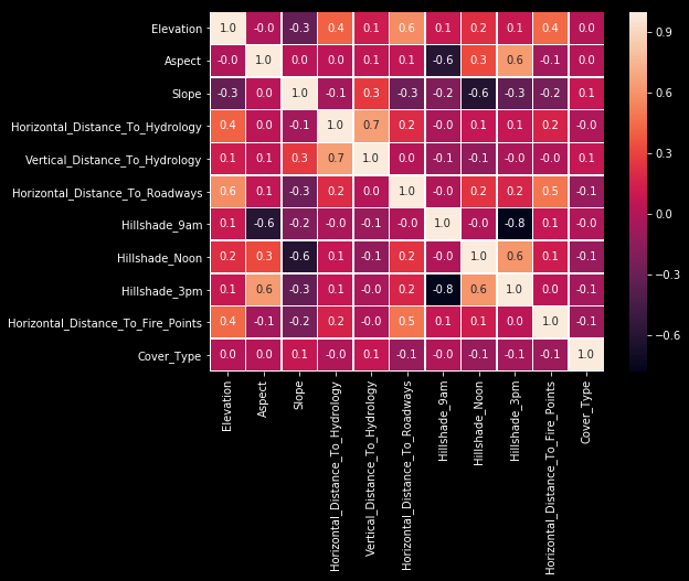
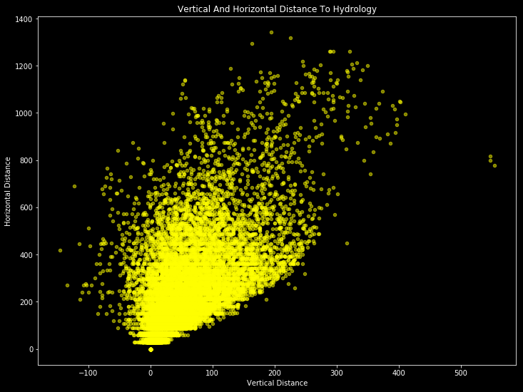
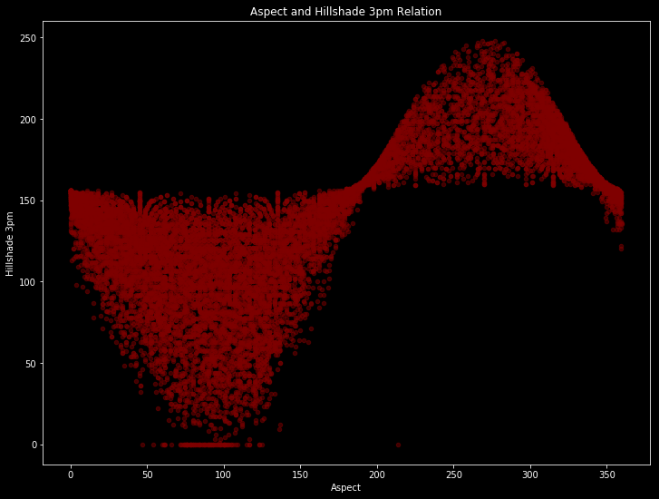
It seems the most important correlations are between “Horizontal Distance To Hydrology” and “Vertical Distance To Hydrology” with 70%; between “Aspect” and “Hillshade 3pm” with 60%; between “Hillshade Noon” and “Hillshade 3pm” with %60; between “Elevation” and “Horizontal Distance To Roadways” with %60. Let’s see how they are looking.
train.plot(kind='scatter', x='Vertical_Distance_To_Hydrology', y='Horizontal_Distance_To_Hydrology', alpha=0.5, color='yellow', figsize = (12,9))
plt.title('Vertical And Horizontal Distance To Hydrology')
plt.xlabel("Vertical Distance")
plt.ylabel("Horizontal Distance")
plt.show()
train.plot(kind='scatter', x='Aspect', y='Hillshade_3pm', alpha=0.5, color='maroon', figsize = (12,9))
plt.title('Aspect and Hillshade 3pm Relation')
plt.xlabel("Aspect")
plt.ylabel("Hillshade 3pm")
plt.show()
train.plot(kind='scatter', x='Hillshade_Noon', y='Hillshade_3pm', alpha=0.5, color='purple', figsize = (12,9))
plt.title('Hillshade Noon and Hillshade 3pm Relation')
plt.xlabel("Hillshade_Noon")
plt.ylabel("Hillshade 3pm")
plt.show()
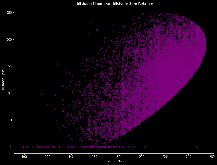
There are obvious patterns if we ignore to outliers. And with this patterns, our model will learn.
Boxplot can be used to see outliers. For a better visualization i will use plotly this time.
Wow, this is very interesting plot! I need to learn this too!
!pip install plotly
Requirement already satisfied: plotly in /usr/local/lib/python3.6/dist-packages (4.1.1)
Requirement already satisfied: six in /usr/local/lib/python3.6/dist-packages (from plotly) (1.12.0)
Requirement already satisfied: retrying>=1.3.3 in /usr/local/lib/python3.6/dist-packages (from plotly) (1.3.3)
import plotly.graph_objs as go
from plotly.offline import iplot

trace1 = go.Box(
    y= train["Vertical_Distance_To_Hydrology"],
    name = 'Vertical Distance',
    marker = dict(color = 'rgb(0,145,119)')
)
trace2 = go.Box(
    y= train["Horizontal_Distance_To_Hydrology"],
    name = 'Horizontal Distance',
    marker = dict(color = 'rgb(5, 79, 174)')
)

data = [trace1, trace2]
layout = dict(autosize=False, width=700,height=500, title='Distance To Hydrology', paper_bgcolor='rgb(243, 243, 243)',
              plot_bgcolor='rgb(243, 243, 243)', margin=dict(l=40,r=30,b=80,t=100,))
fig = dict(data=data, layout=layout)
iplot(fig)
trace1 = go.Box(
    y= train["Hillshade_Noon"],
    name = 'Hillshade Noon',
    marker = dict(color = 'rgb(255,111,145)')
)
trace2 = go.Box(
    y= train["Hillshade_3pm"],
    name = 'Hillshade 3pm',
    marker = dict(color = 'rgb(132,94,194)')
)

data = [trace1, trace2]
layout = dict(autosize=False, width=700,height=500, title='Hillshade 3pm and Noon', paper_bgcolor='rgb(243, 243, 243)',
              plot_bgcolor='rgb(243, 243, 243)', margin=dict(l=40,r=30,b=80,t=100,))
fig = dict(data=data, layout=layout)
iplot(fig)
This time I’ll compare vertical and horizontal distance to hydrology with histogram.
f,ax=plt.subplots(1,2,figsize=(15,7))
train.Vertical_Distance_To_Hydrology.plot.hist(ax=ax[0],bins=30,edgecolor='black',color='crimson')
ax[0].set_title('Vertical Distance To Hydrology')
x1=list(range(-150,350,50))
ax[0].set_xticks(x1)
train.Horizontal_Distance_To_Hydrology.plot.hist(ax=ax[1],bins=30,edgecolor='black',color='darkmagenta')
ax[1].set_title('Horizontal Distance To Hydrology')
x2=list(range(0,1000,100))
ax[1].set_xticks(x2)
plt.show()
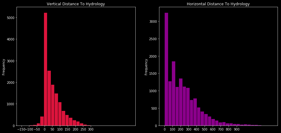
Let’s take a look our categorical categorical variables soil types and wilderness areas.
soil_types = train.iloc[:,14:-1].sum(axis=0)

plt.figure(figsize=(18,9))
sns.barplot(x=soil_types.index, y=soil_types.values, palette="rocket")
plt.xticks(rotation= 75)
plt.ylabel('Total')
plt.title('Count of Soil Types With Value 1',color = 'darkred',fontsize=12)
Text(0.5, 1.0, 'Count of Soil Types With Value 1')
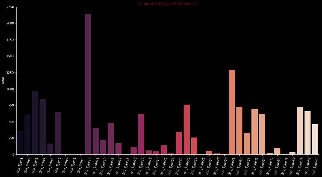
Type 7, Type 8, Type 15 and Type 25 have either no or too few values. Must examine carefully before create a model.
wilderness_areas = train.iloc[:,10:14].sum(axis=0)

plt.figure(figsize=(7,5))
sns.barplot(x=wilderness_areas.index,y=wilderness_areas.values, palette="Blues_d")
plt.xticks(rotation=90)
plt.title('Wilderness Areas',color = 'darkred',fontsize=12)
plt.ylabel('Total')
plt.show()
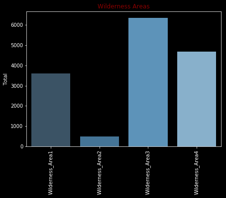
I wonder how many (y) labels we have in each class. I’ll take a look the last column (cover type) for this.
import plotly.express as px

cover_type = train["Cover_Type"].value_counts()
df_cover_type = pd.DataFrame({'CoverType': cover_type.index, 'Total':cover_type.values})

fig = px.bar(df_cover_type, x='CoverType', y='Total', height=400, width=650)
fig.show()
There are same amount of data for each class exactly…
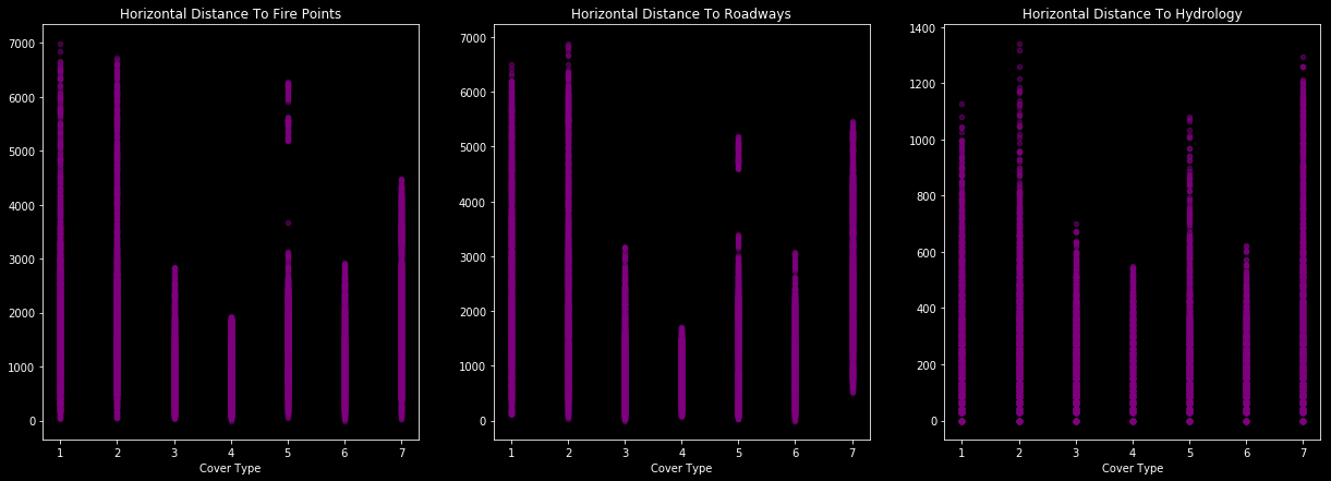
In terms of horizontal distance to x point, distribution of class charts following…
f,ax=plt.subplots(1,3,figsize=(21,7))
train.plot.scatter(ax=ax[0],x='Cover_Type', y='Horizontal_Distance_To_Fire_Points', alpha=0.5, color='purple')
ax[0].set_title('Horizontal Distance To Fire Points')
x1=list(range(1,8,1))
ax[0].set_ylabel("")
ax[0].set_xlabel("Cover Type")
train.plot.scatter(ax=ax[1],x='Cover_Type', y='Horizontal_Distance_To_Roadways', alpha=0.5, color='purple')
ax[1].set_title('Horizontal Distance To Roadways')
x2=list(range(1,8,1))
ax[1].set_ylabel("")
ax[1].set_xlabel("Cover Type")
train.plot.scatter(ax=ax[2],x='Cover_Type', y='Horizontal_Distance_To_Hydrology', alpha=0.5, color='purple')
ax[2].set_title('Horizontal Distance To Hydrology')
x2=list(range(1,8,1))
ax[2].set_ylabel("")
ax[2].set_xlabel("Cover Type")
plt.show()
Pandas Profiling
Actually there is a faster way for exploratory data analysis. Pandas provides you powerful HTML profiling reports with pandas-profiling. It’s like a magic! You can click “Overview”, “Variables” etc tabs for a quick run.
import pandas_profiling as pp

report = pp.ProfileReport(train)
report.to_file("report.html")

report
Modeling
Let’s do it step by step first I’ll slip the training data to make up a validation set and then try out different classification algorithms and then compare them
# Separate the target variable
y = train.Cover_Type
train.drop(['Cover_Type'], axis = 1, inplace = True)
# Split Data
from sklearn.model_selection import train_test_split

train_X, val_X, train_y, val_y = train_test_split(train, y, random_state= 0)

print(f"Train Shape: {train_X.shape}, {train_y.shape}")
print(f"Validation Shape: {val_X.shape}, {val_y.shape}")
Train Shape: (11340, 54), (11340,)
Validation Shape: (3780, 54), (3780,)
# Let's fit the Decision Tree Model first

from sklearn.tree import DecisionTreeClassifier

model = DecisionTreeClassifier()

# Fit the model
model.fit(train_X, train_y)
DecisionTreeClassifier(class_weight=None, criterion='gini', max_depth=None,
                       max_features=None, max_leaf_nodes=None,
                       min_impurity_decrease=0.0, min_impurity_split=None,
                       min_samples_leaf=1, min_samples_split=2,
                       min_weight_fraction_leaf=0.0, presort=False,
                       random_state=None, splitter='best')
# Get predictions for the validation set

predictions = model.predict(val_X)
# Let's check our categorization accuracy

from sklearn.metrics import accuracy_score

accuracy_score(val_y, predictions)
0.7603174603174603
That is good for our first model I know we can improve upon this but let’s see how well we stand on Leaderboard from this very basic model let’s create a submission file and submit the scores and then move on to try different models
# Predict the test data set
predictions_test = model.predict(test)
submission = pd.DataFrame({
    "ID": test.index,
    "Cover_Type": predictions_test
})

submission.to_csv("submission.csv", index = False)
submission.head()
| ID | Cover_Type | |
|---|---|---|
| 0 | 15121 | 1 |
| 1 | 15122 | 1 |
| 2 | 15123 | 1 |
| 3 | 15124 | 1 |
| 4 | 15125 | 1 |
Okay this worked! My score on leaderboard with this was 0.64322 and I received 435th/504 rank Now I’ll try few other models or variations Let’s try Random Forest but first let’s try Decision Tree with some other parameters and let’s see if we can improve our Decision Tree’s accuracy By using all default parameters our Validation Set accuracy is 0.76534
# Let's create a helper function

def calc_tree_accuracy(max_leaf_nodes, train_X, val_X, train_y, val_y):
    model = DecisionTreeClassifier(max_leaf_nodes=max_leaf_nodes, random_state = 0)

    model.fit(train_X, train_y)
    preds = model.predict(val_X)
    acc = accuracy_score(val_y, preds)

    return(acc)
# Now let's fit our model with different max leaf nodes
accuracies = {}
for max_leaf_nodes in range(5, 2000, 50) :
    my_acc = calc_tree_accuracy(max_leaf_nodes, train_X, val_X, train_y, val_y)
    accuracies[max_leaf_nodes] = my_acc
    print(f"Max leaf nodes: {max_leaf_nodes} - - Accuracy: {my_acc}")

print("Best Max Leaf Nodes Parameter:", max(accuracies.items(), key = lambda k : k[1]))
Max leaf nodes: 5 - - Accuracy: 0.557936507936508
Max leaf nodes: 55 - - Accuracy: 0.7092592592592593
Max leaf nodes: 105 - - Accuracy: 0.7394179894179894
Max leaf nodes: 155 - - Accuracy: 0.7497354497354497
Max leaf nodes: 205 - - Accuracy: 0.7579365079365079
Max leaf nodes: 255 - - Accuracy: 0.7584656084656085
Max leaf nodes: 305 - - Accuracy: 0.7619047619047619
Max leaf nodes: 355 - - Accuracy: 0.762962962962963
Max leaf nodes: 405 - - Accuracy: 0.7658730158730159
Max leaf nodes: 455 - - Accuracy: 0.7714285714285715
Max leaf nodes: 505 - - Accuracy: 0.7698412698412699
Max leaf nodes: 555 - - Accuracy: 0.7701058201058201
Max leaf nodes: 605 - - Accuracy: 0.7690476190476191
Max leaf nodes: 655 - - Accuracy: 0.7738095238095238
Max leaf nodes: 705 - - Accuracy: 0.7748677248677248
Max leaf nodes: 755 - - Accuracy: 0.7753968253968254
Max leaf nodes: 805 - - Accuracy: 0.7761904761904762
Max leaf nodes: 855 - - Accuracy: 0.7764550264550265
Max leaf nodes: 905 - - Accuracy: 0.7753968253968254
Max leaf nodes: 955 - - Accuracy: 0.7746031746031746
Max leaf nodes: 1005 - - Accuracy: 0.7738095238095238
Max leaf nodes: 1055 - - Accuracy: 0.773015873015873
Max leaf nodes: 1105 - - Accuracy: 0.7746031746031746
Max leaf nodes: 1155 - - Accuracy: 0.7746031746031746
Max leaf nodes: 1205 - - Accuracy: 0.7711640211640212
Max leaf nodes: 1255 - - Accuracy: 0.7706349206349207
Max leaf nodes: 1305 - - Accuracy: 0.7695767195767196
Max leaf nodes: 1355 - - Accuracy: 0.7674603174603175
Max leaf nodes: 1405 - - Accuracy: 0.7666666666666667
Max leaf nodes: 1455 - - Accuracy: 0.7669312169312169
Max leaf nodes: 1505 - - Accuracy: 0.7653439153439153
Max leaf nodes: 1555 - - Accuracy: 0.7637566137566137
Max leaf nodes: 1605 - - Accuracy: 0.7634920634920634
Max leaf nodes: 1655 - - Accuracy: 0.7603174603174603
Max leaf nodes: 1705 - - Accuracy: 0.7600529100529101
Max leaf nodes: 1755 - - Accuracy: 0.7600529100529101
Max leaf nodes: 1805 - - Accuracy: 0.7600529100529101
Max leaf nodes: 1855 - - Accuracy: 0.7600529100529101
Max leaf nodes: 1905 - - Accuracy: 0.7600529100529101
Max leaf nodes: 1955 - - Accuracy: 0.7600529100529101
Best Max Leaf Nodes Parameter: (855, 0.7764550264550265)
That’s amazing! My accuracy with 5 max leaf nodes was 55% and it kept growing until around max leaf nodes 1705 I think the highest accuracy was around 0.776 at 855 max leaf nodes
# Let's create Random Forest model now
from sklearn.ensemble import RandomForestClassifier

model = RandomForestClassifier(random_state = 0)
model.fit(train_X, train_y)

predictions = model.predict(val_X)

print("Random Forest Accuracy: ", accuracy_score(val_y, predictions))
Random Forest Accuracy:  0.814021164021164


/usr/local/lib/python3.6/dist-packages/sklearn/ensemble/forest.py:245: FutureWarning:

The default value of n_estimators will change from 10 in version 0.20 to 100 in 0.22.
That is a huge improvement! Let’s see where this leads us on the Leaderboard
predictions_test = model.predict(test)
submission = pd.DataFrame({
    "ID": test.index,
    "Cover_Type": predictions_test
})

submission.to_csv("submission.csv", index = False)
Now my score on leaderboard is 0.70138 and ranked 398th out of 505
Let’s try different parameters using grid search cv
%time

from sklearn.model_selection import GridSearchCV

model = RandomForestClassifier(random_state = 0)

param_grid = {
    'n_estimators': [50, 100, 500, 1000],
    'max_features': ['auto', 'sqrt', 'log2'],
    'max_depth' : [8, 9, 10, 11, 12],
    'criterion' :['gini', 'entropy']
}

model_CV = GridSearchCV(estimator = model, param_grid = param_grid, cv = 5)

# We do not need validation set that's why we will train it on full training set
model_CV.fit(train, y)

# Let's check the best parameters
model_CV.best_params_
CPU times: user 0 ns, sys: 2 µs, total: 2 µs
Wall time: 5.48 µs


{'criterion': 'entropy',
 'max_depth': 12,
 'max_features': 'auto',
 'n_estimators': 500}
Okay so let’s train with the best parameters now
model = RandomForestClassifier(random_state=0, max_features='auto', criterion='entropy', max_depth=10, n_estimators=500)

model.fit(train_X, train_y)

predictions = model.predict(val_X)

print("Best Parameters Random Forest Accuracy Is: ", accuracy_score(val_y, predictions))
Best Parameters Random Forest Accuracy Is: 0.7962962962962963
This is almost same or slightly lower than before… Let’s still check on test set
predictions_test = model.predict(test)
submission = pd.DataFrame({
    "ID": test.index,
    "Cover_Type": predictions_test
})

submission.to_csv("submission.csv", index = False)

Leave a comment